POLYFIT Fit Polynomial To Data
Section: Optimization and Curve Fitting
Usage
Thepolyfit routine has the following syntax
p = polyfit(x,y,n)
where x and y are vectors of the same size, and
n is the degree of the approximating polynomial.
The resulting vector p forms the coefficients of
the optimal polynomial (in descending degree) that fit
y with x.
Function Internals
Thepolyfit routine finds the approximating polynomial

such that

is minimized. It does so by forming the Vandermonde matrix
and solving the resulting set of equations using the backslash
operator. Note that the Vandermonde matrix can become poorly
conditioned with large n quite rapidly.
Example
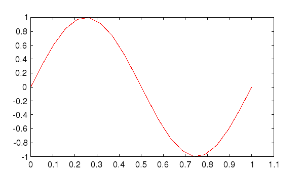
A classic example from Edwards and Penny, consider the problem of approximating a sinusoid with a polynomial. We start with a vector of points evenly spaced on the unit interval, along with a vector of the sine of these points.--> x = linspace(0,1,20); --> y = sin(2*pi*x); --> plot(x,y,'r-')
The resulting plot is shown here
Next, we fit a third degree polynomial to the sine, and use
polyval to plot it
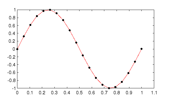
--> p = polyfit(x,y,3)

p =
   21.9170  -32.8756   11.1897   -0.1156

--> f = polyval(p,x);
--> plot(x,y,'r-',x,f,'ko');
The resulting plot is shown here
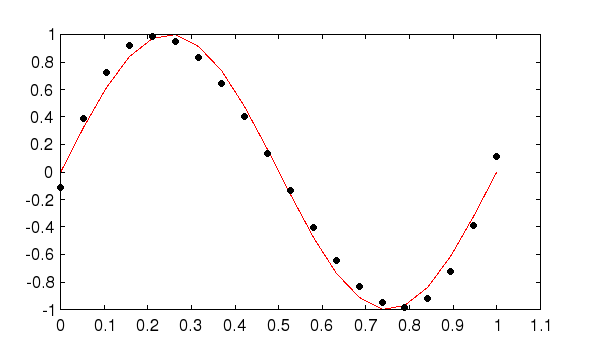
Increasing the order improves the fit, as
--> p = polyfit(x,y,11)

p =

 Columns 1 to 8

   12.4644  -68.5541  130.0555  -71.0940  -38.2814  -14.1222   85.1018   -0.5642

 Columns 9 to 12

  -41.2861   -0.0029    6.2832   -0.0000

--> f = polyval(p,x);
--> plot(x,y,'r-',x,f,'ko');
The resulting plot is shown here