INTERPLIN1 Linear 1-D Interpolation
Section: Optimization and Curve Fitting
Usage
Given a set of monotonically increasingx coordinates and a
corresponding set of y values, performs simple linear
interpolation to a new set of x coordinates. The general syntax
for its usage is
yi = interplin1(x1,y1,xi)
where x1 and y1 are vectors of the same length, and the entries
in x1 are monotoniccally increasing. The output vector yi is
the same size as the input vector xi. For each element of xi,
the values in y1 are linearly interpolated. For values in xi
that are outside the range of x1 the default value returned is
nan. To change this behavior, you can specify the extrapolation
flag:
yi = interplin1(x1,y1,xi,extrapflag)
Valid options for extrapflag are:
-
'nan'- extrapolated values are tagged withnans -
'zero'- extrapolated values are set to zero -
'endpoint'- extrapolated values are set to the endpoint values -
'extrap'- linear extrapolation is performed
x1 and xi vectors must be real, although complex types
are allowed for y1.
Example
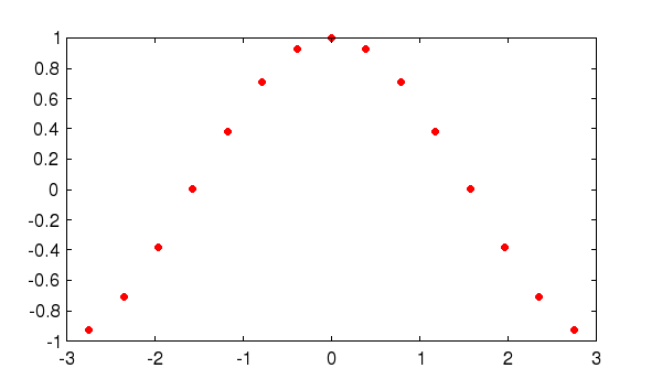
Here is an example of simple linear interpolation with the different extrapolation modes. We start with a fairly coarse sampling of a cosine.--> x = linspace(-pi*7/8,pi*7/8,15); --> y = cos(x); --> plot(x,y,'ro');
which is shown here

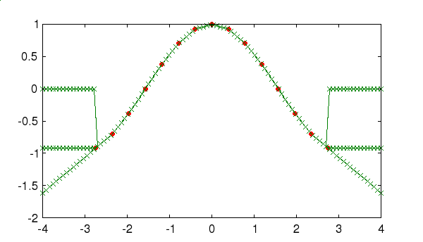
Next, we generate a finer sampling over a slightly broader range
(in this case [-pi,pi]). First, we demonstrate the 'nan'
extrapolation method
--> xi = linspace(-4,4,100);
--> yi_nan = interplin1(x,y,xi,'nan');
--> yi_zero = interplin1(x,y,xi,'zero');
--> yi_endpoint = interplin1(x,y,xi,'endpoint');
--> yi_extrap = interplin1(x,y,xi,'extrap');
--> plot(x,y,'ro',xi,yi_nan,'g-x',xi,yi_zero,'g-x',xi,yi_endpoint,'g-x',xi,yi_extrap,'g-x');
which is shown here

