FreeMat - PLOT Plot Function

PLOT Plot Function

Usage

This is the basic plot command for FreeMat. The general syntax for its use is

  plot(<data 1>,{linespec 1},<data 2>,{linespec 2}...,properties...)

where the <data> arguments can have various forms, and the linespec arguments are optional. We start with the <data> term, which can take on one of multiple forms:

Vector Matrix Case -- In this case the argument data is a pair of variables. A set of x coordinates in a numeric vector, and a set of y coordinates in the columns of the second, numeric matrix. x must have as many elements as y has columns (unless y is a vector, in which case only the number of elements must match). Each column of y is plotted sequentially against the common vector x.
Unpaired Matrix Case -- In this case the argument data is a single numeric matrix y that constitutes the y-values of the plot. An x vector is synthesized as x = 1:length(y), and each column of y is plotted sequentially against this common x axis.
Complex Matrix Case -- Here the argument data is a complex matrix, in which case, the real part of each column is plotted against the imaginary part of each column. All columns receive the same line styles.

Multiple data arguments in a single plot command are treated as a \emph{sequence}, meaning that all of the plots are overlapped on the same set of axes. The linespec is a string used to change the characteristics of the line. In general, the linespec is composed of three optional parts, the colorspec, the symbolspec and the linestylespec in any order. Each of these specifications is a single character that determines the corresponding characteristic. First, the colorspec:

'b' - Color Blue
'g' - Color Green
'r' - Color Red
'c' - Color Cyan
'm' - Color Magenta
'y' - Color Yellow
'k' - Color Black

The symbolspec specifies the (optional) symbol to be drawn at each data point:

'.' - Dot symbol
'o' - Circle symbol
'x' - Times symbol
'+' - Plus symbol
'*' - Asterisk symbol
's' - Square symbol
'd' - Diamond symbol
'v' - Downward-pointing triangle symbol
'^' - Upward-pointing triangle symbol
'<' - Left-pointing triangle symbol
'>' - Right-pointing triangle symbol

The linestylespec specifies the (optional) line style to use for each data series:

'-' - Solid line style
':' - Dotted line style
'-.' - Dot-Dash-Dot-Dash line style
'--' - Dashed line style

For sequences of plots, the linespec is recycled with color order determined by the properties of the current axes. You can also use the properties argument to specify handle properties that will be inherited by all of the plots generated during this event. Finally, you can also specify the handle for the axes that are the target of the plot operation.

  handle = plot(handle,...)

Example

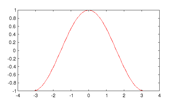
The most common use of the plot command probably involves the vector-matrix paired case. Here, we generate a simple cosine, and plot it using a red line, with no symbols (i.e., a linespec of 'r-').

--> x = linspace(-pi,pi);
--> y = cos(x);
--> plot(x,y,'r-');

which results in the following plot.

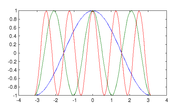
Next, we plot multiple sinusoids (at different frequencies). First, we construct a matrix, in which each column corresponds to a different sinusoid, and then plot them all at once.

--> x = linspace(-pi,pi);
--> y = [cos(x(:)),cos(3*x(:)),cos(5*x(:))];
--> plot(x,y);

In this case, we do not specify a linespec, so that we cycle through the colors automatically (in the order listed in the previous section).

This time, we produce the same plot, but as we want to assign individual linespecs to each line, we use a sequence of arguments in a single plot command, which has the effect of plotting all of the data sets on a common axis, but which allows us to control the linespec of each plot. In the following example, the first line (harmonic) has red, solid lines with times symbols marking the data points, the second line (third harmonic) has blue, solid lines with right-pointing triangle symbols, and the third line (fifth harmonic) has green, dotted lines with asterisk symbols.

--> plot(x,y(:,1),'rx-',x,y(:,2),'b>-',x,y(:,3),'g*:');

The second most frequently used case is the unpaired matrix case. Here, we need to provide only one data component, which will be automatically plotted against a vector of natural number of the appropriate length. Here, we use a plot sequence to change the style of each line to be dotted, dot-dashed, and dashed.

--> plot(y(:,1),'r:',y(:,2),'b;',y(:,3),'g|');

Note in the resulting plot that the x-axis no longer runs from [-pi,pi], but instead runs from [1,100].

The final case is for complex matrices. For complex arguments, the real part is plotted against the imaginary part. Hence, we can generate a 2-dimensional plot from a vector as follows.

--> y = cos(2*x) + i * cos(3*x);
--> plot(y);

Here is an example of using the handle properties to influence the behavior of the generated lines.

--> t = linspace(-3,3);
--> plot(cos(5*t).*exp(-t),'r-','linewidth',3);

FreeMat v4.0 - Online Documentation

PLOT Plot Function

Usage

Example