COLORMAP Image Colormap Function
Section: Handle-Based Graphics
Usage
Changes the colormap for the current figure. The generic syntax for its use iscolormap(map)
where map is a an array organized as 3 \times N),
which defines the RGB (Red Green Blue) coordinates for each color in the
colormap. You can also use the function with no arguments to recover
the current colormap
map = colormap
Function Internals
Assuming that the contents of the colormap function argumentc are
labeled as:

then these columns for the RGB coordinates of pixel in the mapped image. Assume that the image occupies the range $[a,b]$. Then the RGB color of each pixel depends on the value $x$ via the following integer

so that a pixel corresponding to image value $x$ will receive RGB color $[r_k,g_k,b_k]$. Colormaps are generally used to pseudo color images to enhance visibility of features, etc.
Examples
We start by creating a smoothly varying image of a 2D Gaussian pulse.--> x = linspace(-1,1,512)'*ones(1,512); --> y = x'; --> Z = exp(-(x.^2+y.^2)/0.3); --> image(Z);
which we display with the default (grayscale) colormap here.

Next we switch to the copper colormap, and redisplay the image.
--> colormap(copper);
--> image(Z);
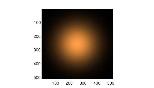
which results in the following image.

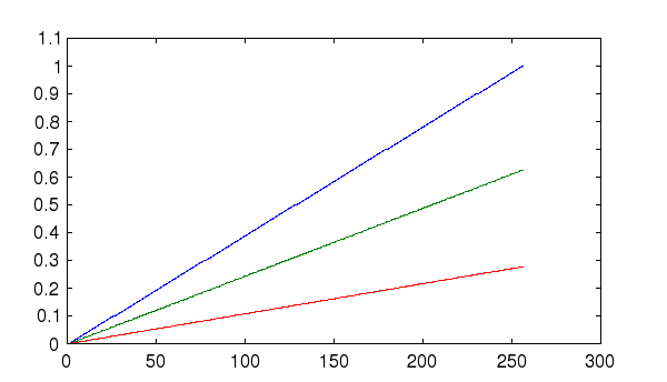
If we capture the output of the copper command and plot it, we obtain
the following result:
--> a = copper;
--> plot(a);

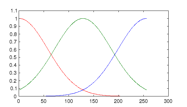
Note that in the output that each of the color components are linear functions of the index, with the ratio between the red, blue and green components remaining constant as a function of index. The result is an intensity map with a copper tint. We can similarly construct a colormap of our own by defining the three components seperately. For example, suppose we take three gaussian curves, one for each color, centered on different parts of the index space:
--> t = linspace(0,1,256);
--> A = [exp(-(t-1.0).^2/0.1);exp(-(t-0.5).^2/0.1);exp(-t.^2/0.1)]';
--> plot(A);

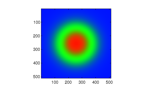
The resulting image has dark bands in it near the color transitions.
--> image(Z);
--> colormap(A);

These dark bands are a result of the nonuniform color intensity, which we can correct for by renormalizing each color to have the same norm.
--> w = sqrt(sum(A'.^2));
--> sA = diag(1./w)*A;
--> plot(A);

The resulting image has no more dark bands.
--> image(Z);
--> colormap(A);

